1.Overview
We described copy number variation analysis workflow here based on copy number variation analysis pipeline[1] by Genome Data Commons (GDC). We also referenced copy number inference pipeline[2] by GenePattern. We showed a tumor-normal different CNV analysis workflow via public TCGA breast cancer (BRCA) CNV paired-sample data derived from Affymetrix SNP 6.0 array data. The raw .CEL files depict SNP and CNV intensity measurements by probes from Affymetrix SNP 6.0 array. Firstly, Birdsuite is used for the normalization of raw data and the estimation of raw copy number. Secondly, processed data is transmitted to DNAcopy R package for circular binary segmentation (CBS) analysis. CBS method outputs contiguous chromosome regions with estimated copy number for each region. Thirdly, GISTIC 2.0 takes the output file of DNAcopy as input and mainly generates a genotype file showing CNV located in gene for each sample, a file depicting G-score and q-value for the significant level of CNV and several graphs showing the location of copy number deletion and amplification in the human genome. Finally, hypothesis test for the selection of different genes with CNV and function analysis of different genes are processed.
2.Data sets
Owing to the inaccessibility of TCGA level 1 and level 2 data for public, we downloaded publicly available TCGA level 3 sample data, that is, copy number segment file. Users could directly download in the GDC Data Portal website[3]. Users also obtain data from GDC via tools such as R package (TCGAbiolinks[4], etc.) and Data Transfer Tool[5]. Here, we used R package TCGAbiolinks to download TCGA breast cancer (BRCA) level 3 data generated by Hg38 reference genome.
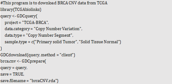
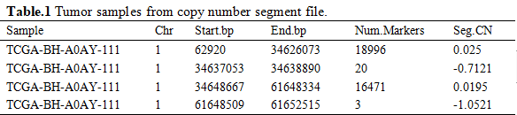
Subsequently, we transferred origin data into paired sample datasets that tumor tissue and normal tissue are from a identical sample via TCGA database sample ID. We divided samples into tumor group and normal group, which are shown below (Table.1).
3.Tumor-normal CNV difference analysis
3.1 Processing data by GITSIC 2.0
We used the online version of GISTIC 2.0[6] at GenePattern[7] (Figure.1) and chose the Hg38 reference genome to process copy number files respectively. Notably, the marker file is not necessary and other parameters are staying default. It took about half an hour to an hour. If you use marker file, you could download the probe-set for the GRCh38 reference genome[8]. Additionally, the online version of GISTIC 2.0 provides instruction of usage[9].
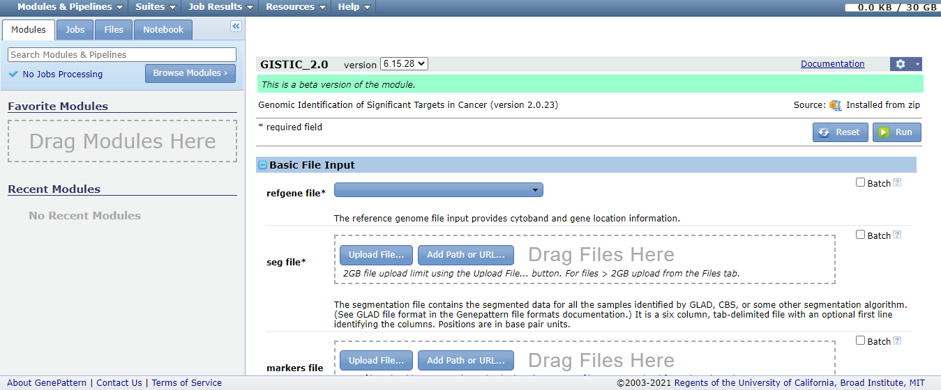
Figure.1 The interface of the online version of GISTIC 2.0. The symbols of ‘*’ represent the required items. Users could choose refgene file parameter including Hg18, Hg19 and Hg38 refgene files. Copy number segment file needs to be uploaded.
3.2 Output of GITSIC 2.0
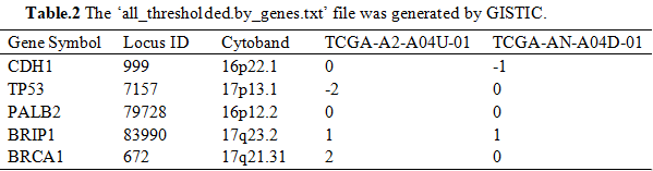
There were 19 files as output (Figure.2). Among these files, GISTIC 2.0 visualized raw copy number and the location of CNV in the human genome respectively, deletions and amplifications (Figure.3). Additionally, a genotype file (all_thresholded.by_genes.txt) shows CNV located in gene for each sample, a file depicting G-score and q-value for the significant level of CNV.
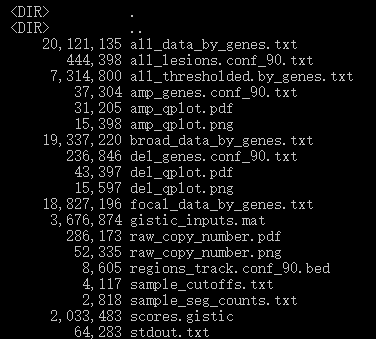
Figure.2 The 19 output files generated by GISTIC were shown.
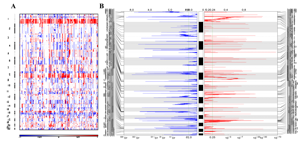
Figure.3 The visualization output of GISTIC. A. The heatmap of the raw copy number from tumor samples. B. The combination of plots depicting copy number deletions and amplifications.
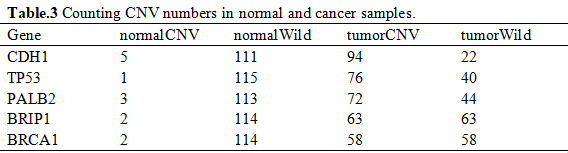
3.3 Hypothesis test
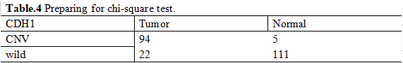
Subsequently, we used one-marker test for the selection of different genes with CNV. Firstly, counting CNV numbers in normal and cancer samples, respectively (Table.3). Applying chi-square test for the association between CNV and cancer for each gene (Table.4).
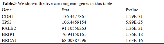
After hypothesis test, we selected 5812 genes by the cutoff of 2.2 × 10⁻¹⁶ (Table.5).
Subsequently, we visualized the distribution of different genes with copy number gain or loss in the human genome (Figure.3).
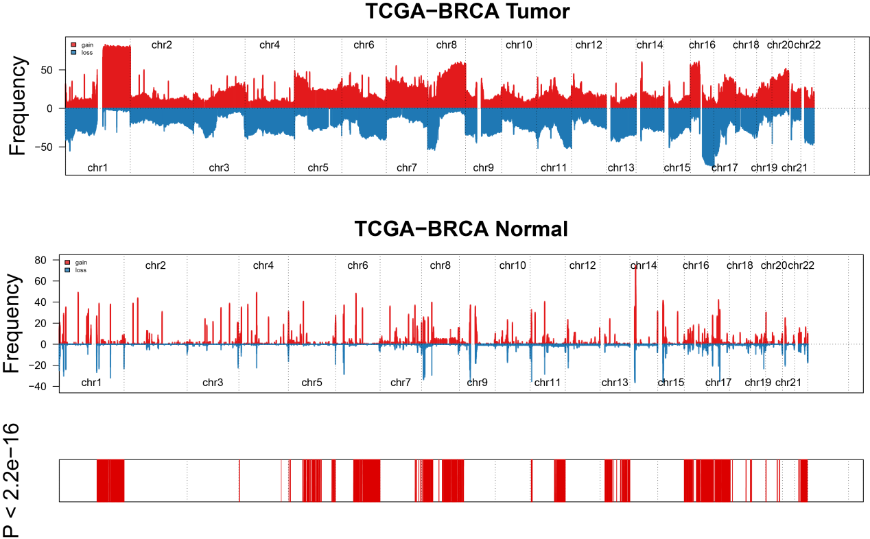
Figure.4 Genome features in tumor and normal groups. We chose 5812 different genes by the cutoff of 2.2 × 10⁻¹⁶ after chi-square test and showed the distribution of copy number gain or loss in the 22 human chromosomes in tumor and normal samples. Amplification of genes is marked in blue. Deletion of genes is narked in red.
3.4 Function analysis
Finally, we used R package clusterProfilter [10] for the GO and KEGG annotation of 5812 significantly different genes. We respectively selected the top 10 significant pathways for display (Figure.5).
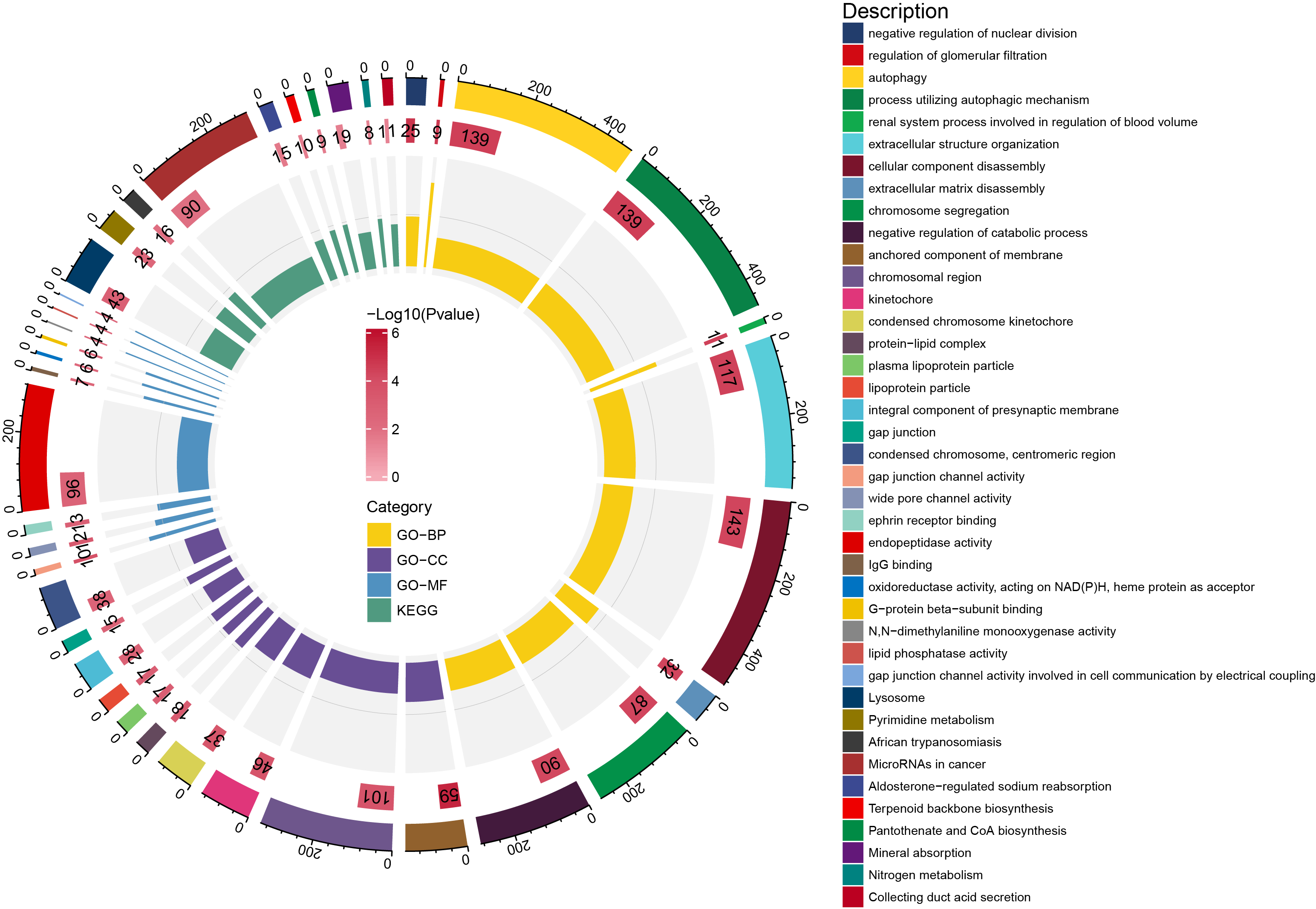
Figure.5 We depicted the GO and KEGG significantly pathways associated with different genes.
4.Reference
[1] Copy Number Variation Analysis Pipeline. https://docs.gdc.cancer.gov/Data/Bioinformatics_Pipelines/CNV_Pipeline/
[2] Affymetrix SNP6 Copy Number Inference Pipeline. https://genepattern.org/affymetrix-snp6-copy-number-inference-pipeline.
[3] Genomic Data Commons Data Portal. https://portal.gdc.cancer.gov/.
[4] A. Colaprico, T.C. Silva, C. Olsen, L. Garofano, C. Cava, D. Garolini, T.S. Sabedot, T.M. Malta, S.M. Pagnotta, I. Castiglioni, M. Ceccarelli, G. Bontempi, H. Noushmehr, TCGAbiolinks: an R/Bioconductor package for integrative analysis of TCGA data, Nucleic acids research 44(8) (2015) e71-e71.
[5] GDC Data Transfer Tool. https://gdc.cancer.gov/access-data/gdc-data-transfer-tool.
[6] C.H. Mermel, S.E. Schumacher, B. Hill, M.L. Meyerson, R. Beroukhim, G. Getz, GISTIC2.0 facilitates sensitive and confident localization of the targets of focal somatic copy-number alteration in human cancers, Genome biology 12(4) (2011) R41.
[7] M. Reich, T. Liefeld, J. Gould, J. Lerner, P. Tamayo, J.P. Mesirov, GenePattern 2.0.
[8] GDC Reference File Website. https://gdc.cancer.gov/about-data/gdc-data-processing/gdc-reference-files.
[9] GISTIC2 Documentation. https://genepattern.org/doc/GISTIC_2.0/2.0.23/GISTICDocumentation_standalone.htm.
[10] G. Yu, L.G. Wang, Y. Han, Q.Y. He, clusterProfiler: an R package for comparing biological themes among gene clusters, Omics : a journal of integrative biology 16(5) (2012) 284-7.